Stardis: Starter Pack

The Stardis: Starter Pack is a collection of input data sets ready for use with stardis, over a few examples. It also provides POSIX shell scripts that make easier the invocation of the stardis program. It gives an overview of the required input data and the features of stardis.

Illustration of the infrared rendering of the porous example supplied in the Starter Pack. The color map displays the temperature in Kelvin. The animation was produced by a simple rotation of the camera around the center of the foam. Each one of the 32 frames is a full image produced by a Stardis run.

Downloads

Version	Archive
0.2.1	[tarball] [pgp]

Quick start

Assuming that stardis is correctly installed and registered against your current POSIX shell, simply run the POSIX shell script of the example that you want to run. For instance:

~/Stardis-StarterPack $ cd heatsink
~/Stardis-StarterPack/heatsink $ sh run_medium_computation.sh

On script invocation, stardis is ran according to the data of the example and the simulation parameters defined in the USER PARAMETERS section of the script. Each example and its launching script is explained hereafter.

Content

The cube

This example is simply a cube of solid with a constant source term in the whole volume. Only thermal conduction is considered in this example. The interest of this example is to be able to compare with an unstationary analytical solution.

The 3 provided POSIX shell scripts illustrate 3 main features of Stardis: the probe computation, the visualization of thermal paths and the Green function evaluation.

Geometric data and physical properties

The geometric data are described in ASCII STL format. The cube is provided in the solid.stl file. If you visualize the stl file with a software like paraview or meshlab, you can see that the cube is described by a basic triangulation. Stardis does not require a fine meshing: the computation is not based on any geometrical meshing; the STL file must only describe the boundary of a solid.

You can see three other STL files: left_bc.stl, right_bc.stl and center_bc.stl. These files are required to attach boundary conditions to the geometry. We note an important constraint in the CAD process: the triangles in these boundary STL files which coincide with the triangles in the solid STL files must be rigorously the same. This conformal mesh constraint is also required for adjacent solids that share a common interface.

Finally you can have a look at the model.txt file which is the stardis input data file. In this file we connect:

physical properties (thermal conductivity, thermal capacity, ...) to the geometrical data (here solid.stl only);
boundary conditions to the geometrical data. You can see here a fixed temperature (Dirichlet boundary condition) is applied to the boundaries represented by right_bc.stl and left_bc.stl, and a null flux condition is applied to the boundaries represented by center_bc.stl (adiabatic boundaries).

You can refer to the stardis-input man page to read this file and modify it as you wish.

Probe computation

The script run_probe_computation.sh invokes the stardis program in order to compute the temperature at the center of the cube for different values of time. The results will be recorded in a file and plotted with gnuplot (provided it has been installed), in order to compare results obtained by stardis to the analytical solution stored in the analytical_T.txt file.

Assuming the current shell directory is ~/Stardis-StarterPack/cube and that the stardis program is registered against the current shell, you can run the script using the following command:

~/Stardis-StardisPack/cube $ sh ./run_probe_computation.sh

You can also simply invoke the stardis program in order to compute the temperature at the center of the cube at steady state, by using the following command:

~/Stardis-StarterPack/cube $ stardis -M model.txt -p 0.5,0.5,0.5 -e

Please refer to the stardis man page for an explanation about command-line options. The shell script can be edited and modified. For instance, in section USER PARAMETERS, the number of Monte-Carlo samples or the value of the probe time can be changed.

Dump some "thermal paths"

The script run_dump_paths.sh invokes stardis twice:

first to dump the scene in the vtk format. This feature is useful for checking the integrity of the geometrical data. For instance if the STL files provide a non-conformal triangle mesh, some errors will be mentioned in the vtk file.
to produce some "thermal paths", starting from the probe position and time. Visualising these paths provides useful information about the boundary or initial conditions that are involved for the computation of the probe temperature, as well as their relative importance. This example is simple but yet allows the visualization of thermal paths in a complex geometry where radiative, convective and conductive heat transfers are coupled.

You can modify the number of paths or the probe position by editing the script.

Green function evaluation

The last script run_green_evaluation.sh shows how to estimate the Green function with stardis and how to use it with the sgreen program. On first invocation, the script runs stardis to evaluate the Green function by generating the required number of thermal paths and store some data (the end position of each path) in a binary file. This Green function is evaluated for the probe position defined in the USER PARAMETERS SECTION.

This Green function is independent of the value of the sources (values of boundary and initial conditions, as well as the volumetric source term). If you launch the script again, the sgreen program will process the Green function to compute the probe temperature, for the current values of sources (no matter whether they have been modified or not); in order to modify the values of the sources, the following line should be modified in the script:

SOURCES_AND_BOUNDARIES="CUBE.VP=12 LTEMP.T=290 RTEMP.T=310 ADIA.F=5.2"

with CUBE.VP the value of the volumetric source term (in W/m^3); LTEMP.T and RTEMP.T the values of the temperature on the left (LTEMP) and right (RTEMP) boundaries respectively (in K); and ADIA.F the value of the heat flux density imposed to the boundary ADIA (in W/m^2). The names of the sources (here CUBE, RTEMP, LTEMP and ADIA) are simply the names used in the model.txt file.

Please note that ADIA being a boundary of type flux (defined by the F_BOUNDARY_FOR_SOLID keyword in the model.txt file) the corresponding source value is named ADIA.F and not ADIA.T as for boundaries of type temperature.

The heatsink

This example is more complex than the previous one. It represents an electronic chip with its heatsink. As mentioned in the model.txt file, the model is composed of three media: the heasink, the chip that produces heat and an interface material between the heatsink and the chip.

The run_medium_computation.sh script launches stardis to compute the mean temperature in the chip at steady state. It will also create the geometry in vtk format.

The run_medium_computation_multiple.sh script does the same computation for the model described in file model_multiple.txt. While this is an assembly of 50 similar electronic devices, the computation time will not be 50 times greater: it will be of the same order of magnitude.

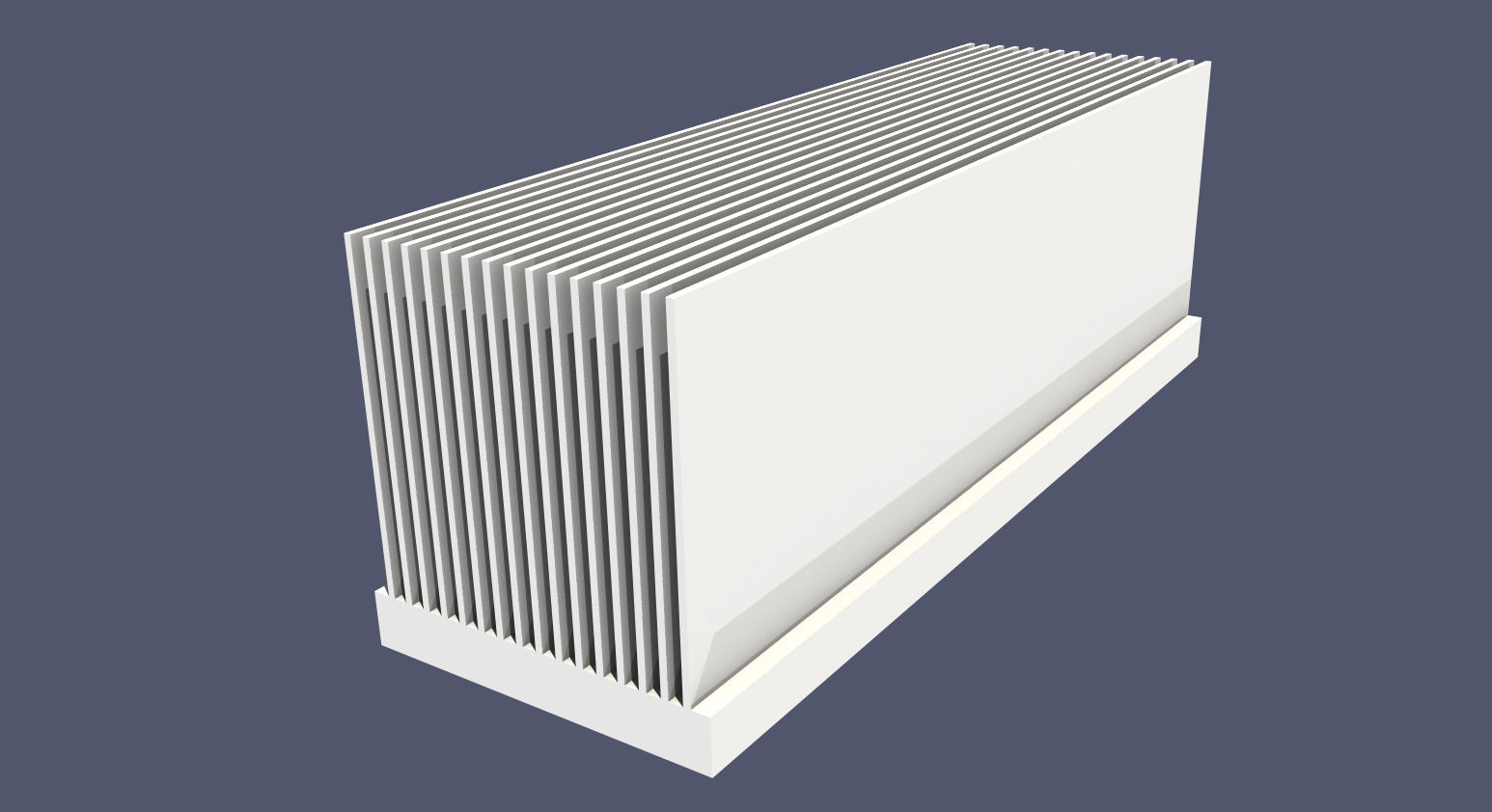
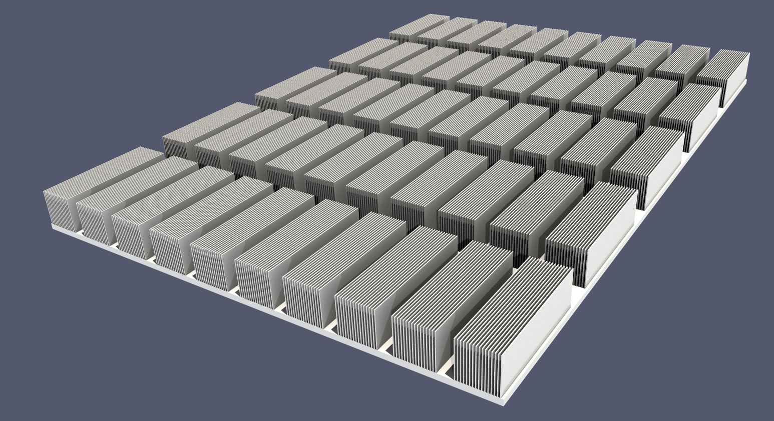
Geometry of the heat sink test cases

The porous medium

In this example, we show an original feature: infrared rendering. stardis is able to render a scene in infrared without prior knowledge of the temperature field.

The run_IR_rendering.sh script provides an example to launch stardis in rendering mode. The scene is an idealized porous medium above a reflective plane. Some parameters can be modified in the USER PARAMETERS section, such as the resolution of the image and the number of samples per pixel. For each pixel of the image, the luminance is computed by Monte-Carlo and the number of realizations is the specified number of samples per pixel. Computing a high-definition image with little statistical noise can therefore take a long time (many hours). The values of the parameters provided in the script should result in a computation time of about a dozen minutes on a recent low-end desktop computer.

More information about the rendering is provided in the stardis man page (such as the parameters associated with the point of view).

Acknowledgement to Cyril Caliot who designed the porous model for the Optisol project (ANR-11-SEED-0009, PROMES-CNRS, CIRIMAT, SICAT, LTN). This model represents an ideal metallic or SiC foam. This type of foam is used in the design of heat exchangers in concentrated solar processes in order to transfer incoming solar radiation energy to a working fluid.

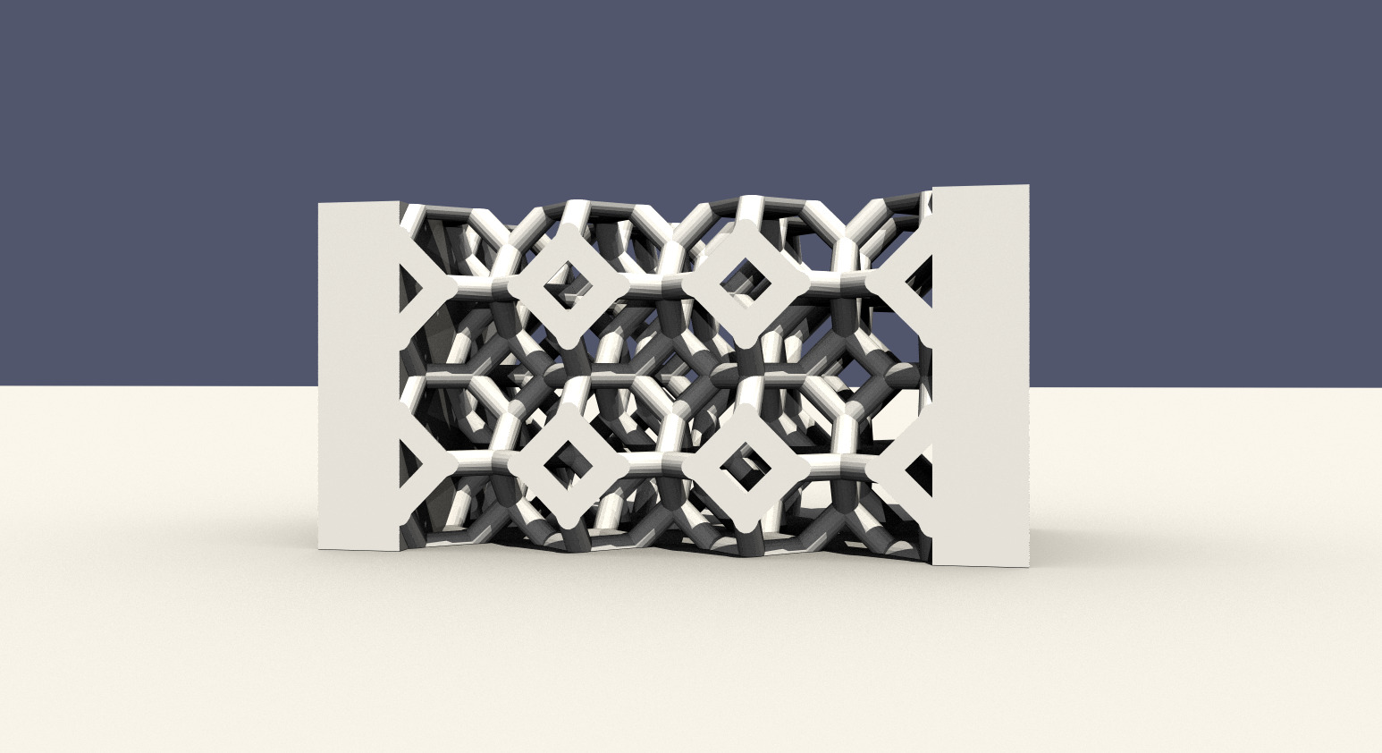
Geometry of the porous example. It is in fact a foam composed of a set of kelvin cells.

The city

This last example shows the ability to deal with geometrical small-scale details in a larger scene. The scene is a pseudo-realistic city composed of buildings with geometrical details like glazing (~ 24 mm width), internal insulation and balconies.

An infrared rendering of this scene illustrates typical thermal bridges in a building, at floor-wall junctions and balcony-floor junctions. And for didactic reasons, there is no insulation of the roof.

The rendering is obtained at steady state with a known external air temperature of 0°C and a known internal air temperature of 20°C (which is a simple model for a perfect heating system). The temperature field is unknown at any position in the buildings and in the ground. The temperature is set at 13°C at a depth of 5 meters. We have also added a "lake" (modeled as a reflecting solid) in front of the buildings to get some specular reflection.

As for the previous example, the run_IR_rendering.sh script provides an example to launch stardis in rendering mode and some parameters can be modified in the USER PARAMETERS section. With the default parameters, the computation time may take several hours.

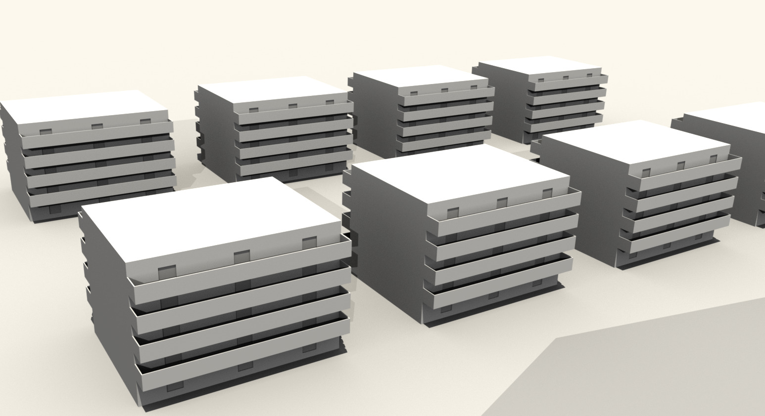
Geometry of the "city" test case. Each building is fully described, from balconies and rooms to walls, foundations, floors and insulation.

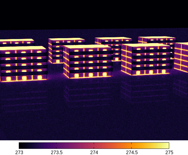
Infrared rendering of the “city” test case illustrating thermal bridges, particularly those coming from the uninsulated roofs. The color map displays the temperature in Kelvin.

Release notes

Version 0.2.1

Fix several scripts that were not working properly with Stardis 0.12.
Update the radiative ambient temperature of the urban scene. It had been set to 300 K, which did not match the originally planned configuration, which called for a temperature of 273 K. The resulting image was therefore saturated: all displayed temperatures exceeded the expected range of 273 to 275 K.

Version 0.2

Updates input files to make them compatible with file format updates introduced by Stardis 0.8.
Make script shells POSIX compliant.

Version 0.1

Add the city exemple

Copyright notice

License

Stardis: Starter Pack is free software released under the GPLv3+ license: GNU GPL version 3 or later. You can freely study, modify or extend it. You are also welcome to redistribute it under certain conditions; refer to the license for details.